Mind Your Metals: Exploring the Impact of Heavy Metals on Depression with Machine Learning
National Health and Nutrition Examination Survey 2005-2006
The National Health and Nutrition Examination Survey (NHANES) is a large and comprehensive dataset that includes information about the health and nutrition status of individuals in the United States. The 2005-2006 dataset (ICPSR 25504) is a nationally representative sample of individuals aged 6 months and older who participated in the survey between 2005 and 2006.
The dataset includes a wide range of variables, including demographic information (age, sex, race/ethnicity, education level), health status (including chronic health conditions and health behaviors such as smoking and physical activity), and measures of nutrition and dietary intake (such as calorie and nutrient intake, dietary patterns, and food frequency). There are also physical measurements such as blood pressure, body mass index (BMI), and waist circumference.
The dataset can be used to answer a wide range of research questions related to public health and nutrition. Some potential insights that can be gained from exploring the dataset include:
The prevalence of chronic health conditions such as hypertension, diabetes, and obesity in different demographic groups
The associations between health behaviors (such as smoking and physical activity) and health outcomes
The dietary patterns and nutrient intake of different demographic groups
The relationships between nutrition and health outcomes such as cardiovascular disease and diabetes
The associations between physical measurements such as BMI and waist circumference and health outcomes
Exploring these and other questions can provide valuable insights into the health status of different populations and can inform public health policies and interventions aimed at improving health outcomes.
Mind Your Metals: Exploring the Impact of Heavy Metals on Depression with Machine Learning
The association between heavy metals and depression has been a topic of interest in scientific research. Studies have investigated the potential relationship between exposure to heavy metals and the development or exacerbation of depressive symptoms. Here are some general observations from the existing literature:
Lead: Exposure to lead has been associated with an increased risk of depressive symptoms. Lead is a neurotoxic metal that can affect the central nervous system and disrupt neurotransmitter function, potentially contributing to depressive symptoms.
Mercury: Some studies suggest a possible link between mercury exposure and depression. Mercury is a toxic metal that can accumulate in the body, including the brain. It may have adverse effects on mood regulation and neurotransmitter function, potentially contributing to depressive symptoms.
Cadmium: Cadmium exposure has been associated with an increased risk of depression in some studies. Cadmium is a toxic metal found in industrial pollutants and tobacco smoke. It may disrupt neuroendocrine function and contribute to the development of depressive symptoms.
Machine Learning within Studies of Early-life Environmental Exposures and Child Health: Review of the current literature and discussion of next-steps
Oskar and Stingone emphasize that while ML methods have been widely used for prediction and classification in other fields, environmental health research has traditionally focused on causal or explanatory modeling. However, with the availability of complex environmental health data and the interest in holistic exposure paradigms such as the exposome, there is a need for analytic methods that can address the unique challenges posed by high-dimensional environmental health data.
Their article explores how researchers have applied ML methods in studies of environmental exposures and childrens’ health. It identifies common themes in these studies, including the analysis of environmental mixtures, exposure prediction and characterization, disease prediction and forecasting, analysis of other complex data, and improvements to causal inference. The review summarizes the strengths and limitations of implementing ML methods in these areas and identifies gaps in the literature.
Machine learning model for depression based on heavy metals among aging people: A study with National Health and Nutrition Examination Survey 2017–2018
Xia et al. aimed to explore the association between depression and blood metal elements using a machine learning model. The study utilized data from the National Health and Nutrition Examination Survey (NHANES) conducted in 2017-2018. A total of 3,247 aging samples were included, and 10 different metals were analyzed, including lead (Pb), mercury (Hg), cadmium (Cd), manganese (Mn), selenium (Se), chromium (Cr), cobalt (Co), inorganic mercury (InHg), methylmercury (MeHg), and ethyl mercury (EtHg).
The study compared eight machine learning algorithms for analyzing the association between metal elements and depression. Among the algorithms tested, XGBoost showed optimal effects and was used for further analysis. The study employed both Poisson regression and the XGBoost model to identify risk factors and predict depression.
The results revealed that out of the 3,247 participants, 344 individuals were diagnosed with depression. In the Poisson regression model, the metals Cd (β = 0.22, P = 0.00000941), EtHg (β = 3.43, P = 0.003216), and Hg (β = -0.15, P = 0.001524) were found to be significantly related to depression. The XGBoost model demonstrated good performance for evaluating depression, with an accuracy of 0.89 (95%CI: 0.87, 0.92), a Kappa value of 0.006, and an area under the curve (AUC) of 0.88. An online XGBoost application for depression prediction was also developed.
The study concluded that blood heavy metals, particularly Cd, EtHg, and Hg, were significantly associated with depression. The prediction of depression using machine learning models was deemed essential.
Association of urinary heavy metals co-exposure and adult depression: Modification of physical activity
Fu et al. aimed to investigate the association between exposure to a mixture of urinary heavy metals and depression, as well as the potential moderating role of physical activity in this relationship. The study used data from the National Health and Nutrition Examination Survey (NHANES) conducted between 2011 and 2016. Depression was assessed using the Patient Health Questionnaire. Elastic net regression was used to select six heavy metals (cadmium, cobalt, tin, antimony, thallium, and mercury) for further analysis. Binomial logistic regression, generalized additive models, environment risk score (ERS), and weighted quantile sum (WQS) regression were employed to examine the effects of individual and cumulative exposure to these metals on depression risk. The study included 4,212 participants, and the prevalence of depression was 7.40%.
The findings of the study indicated that urinary tin and antimony exposure were independently associated with an increased risk of depression. A linear dose-response relationship between tin exposure and depression risk was also observed. Moreover, cumulative exposure to multiple heavy metals was positively associated with depression risk, with tin, antimony, and cadmium identified as the metals contributing most to the overall mixture effect. Notably, the significant positive association between heavy metal mixture exposure and depression risk was observed primarily in individuals who were inactive in physical activity.
In conclusion, this study demonstrated that combined exposure to urinary heavy metals was associated with an increased risk of depression. However, the detrimental effects of heavy metal exposure on depression risk appeared to be attenuated by engaging in physical activity. These findings have important implications for public health, highlighting the potential role of both heavy metal exposure and physical activity in the development and prevention of depression.
Research Question:
Mind Your Metals aims to predict how factors such as age, gender, and heavy metals(lead, cadmium, and mercury etc.) can have an affect on one’s mental health, specifically depression. We will examine this topic as a classification problem.
From the National Health and Nutrition Examination Survey we chose to examine:
Independent Variable(s):
DS1: Demographics
Age
Gender
DS102: Blood Lead and Blood Cadmium
Lead
Cadmium
DS130: Blood Total Mercury and Blood Total Inorganic Mercury
   SEQN                        SDDSRVYR                          RIDSTATR
1 31127 NHANES 2005-2006 Public Release Both Interviewed and MEC examined
2 31128 NHANES 2005-2006 Public Release Both Interviewed and MEC examined
3 31129 NHANES 2005-2006 Public Release Both Interviewed and MEC examined
4 31130 NHANES 2005-2006 Public Release Both Interviewed and MEC examined
5 31131 NHANES 2005-2006 Public Release Both Interviewed and MEC examined
6 31132 NHANES 2005-2006 Public Release Both Interviewed and MEC examined
                     RIDEXMON RIAGENDR RIDAGEYR RIDAGEMN RIDAGEEX
1    May 1 through October 31     Male        0       11       12
2 November 1 through April 30   Female       11      132      132
3    May 1 through October 31     Male       15      189      190
4    May 1 through October 31   Female       85       NA       NA
5    May 1 through October 31   Female       44      535      536
6    May 1 through October 31     Male       70      842      843
            RIDRETH1 DMQMILIT                                DMDBORN
1 Non-Hispanic White     <NA> Born in 50 US States or Washington, DC
2 Non-Hispanic Black     <NA> Born in 50 US States or Washington, DC
3 Non-Hispanic Black     <NA> Born in 50 US States or Washington, DC
4 Non-Hispanic White       No Born in 50 US States or Washington, DC
5 Non-Hispanic Black       No Born in 50 US States or Washington, DC
6 Non-Hispanic White      Yes Born in 50 US States or Washington, DC
                            DMDCITZN DMDYRSUS   DMDEDUC3
1 Citizen by birth or naturalization     <NA>       <NA>
2 Citizen by birth or naturalization     <NA>  4th Grade
3 Citizen by birth or naturalization     <NA> 10th Grade
4 Citizen by birth or naturalization     <NA>       <NA>
5 Citizen by birth or naturalization     <NA>       <NA>
6 Citizen by birth or naturalization     <NA>       <NA>
                   DMDEDUC2  DMDSCHOL      DMDMARTL DMDHHSIZ DMDFMSIZ
1                      <NA>      <NA>          <NA>        4        4
2                      <NA> In school          <NA>        7        6
3                      <NA> In school Never married        6        6
4 Some College or AA degree      <NA>       Widowed        1        1
5 Some College or AA degree      <NA>       Married        4        4
6 College Graduate or above      <NA>       Married        2        2
            INDHHINC           INDFMINC INDFMPIR                RIDEXPRG
1 $15,000 to $19,999 $15,000 to $19,999     0.75                    <NA>
2 $45,000 to $54,999 $20,000 to $24,999     0.77 SP not pregnant at exam
3 $65,000 to $74,999 $65,000 to $74,999     2.71                    <NA>
4 $15,000 to $19,999 $15,000 to $19,999     1.99                    <NA>
5   $75,000 and Over   $75,000 and Over     4.65 SP not pregnant at exam
6   $75,000 and Over   $75,000 and Over     5.00                    <NA>
  DMDHRGND DMDHRAGE                               DMDHRBRN
1   Female       21 Born in 50 US States or Washington, DC
2     Male       47 Born in 50 US States or Washington, DC
3     Male       41 Born in 50 US States or Washington, DC
4   Female       85 Born in 50 US States or Washington, DC
5     Male       36 Born in 50 US States or Washington, DC
6     Male       70 Born in 50 US States or Washington, DC
                                            DMDHREDU DMDHRMAR
1                 High School Grad/GED or equivalent  Married
2 9-11th Grade (Includes 12th grade with no diploma)     <NA>
3                          Some College or AA degree  Married
4                          Some College or AA degree  Widowed
5                          College Graduate or above  Married
6                          College Graduate or above  Married
                                            DMDHSEDU SIALANG SIAPROXY SIAINTRP
1 9-11th Grade (Includes 12th grade with no diploma) English      Yes       No
2                                               <NA> English      Yes       No
3                          Some College or AA degree English      Yes       No
4                                               <NA> English       No       No
5                          Some College or AA degree English       No       No
6                          College Graduate or above English       No       No
  FIALANG FIAPROXY FIAINTRP MIALANG MIAPROXY MIAINTRP AIALANG  WTINT2YR
1 English       No       No    <NA>     <NA>     <NA>    <NA>  6434.950
2 English       No       No English       No       No English  9081.701
3 English       No       No English       No       No English  5316.895
4 English       No       No    <NA>     <NA>     <NA>    <NA> 29960.840
5 English       No       No English       No       No English 26457.708
6 English       No       No English       No       No English 32961.510
   WTMEC2YR SDMVPSU SDMVSTRA
1  6571.396       2       44
2  8987.042       1       52
3  5586.719       1       51
4 34030.995       2       46
5 26770.585       1       48
6 35315.539       2       52
   SEQN LBXBCD LBDBCDSI LBXBPB LBDBPBSI                        SDDSRVYR
1 31128   0.14     1.25   2.24    0.108 NHANES 2005-2006 Public Release
2 31129   0.24     2.14   0.32    0.015 NHANES 2005-2006 Public Release
3 31130     NA       NA     NA       NA NHANES 2005-2006 Public Release
4 31131   0.14     1.25   1.01    0.049 NHANES 2005-2006 Public Release
5 31132   0.14     1.25   1.86    0.090 NHANES 2005-2006 Public Release
6 31133   0.26     2.31   0.35    0.017 NHANES 2005-2006 Public Release
                           RIDSTATR                    RIDEXMON RIAGENDR
1 Both Interviewed and MEC examined November 1 through April 30   Female
2 Both Interviewed and MEC examined    May 1 through October 31     Male
3 Both Interviewed and MEC examined    May 1 through October 31   Female
4 Both Interviewed and MEC examined    May 1 through October 31   Female
5 Both Interviewed and MEC examined    May 1 through October 31     Male
6 Both Interviewed and MEC examined    May 1 through October 31   Female
  RIDAGEYR RIDAGEMN RIDAGEEX           RIDRETH1 DMQMILIT
1       11      132      132 Non-Hispanic Black     <NA>
2       15      189      190 Non-Hispanic Black     <NA>
3       85       NA       NA Non-Hispanic White       No
4       44      535      536 Non-Hispanic Black       No
5       70      842      843 Non-Hispanic White      Yes
6       16      193      194 Non-Hispanic Black     <NA>
                                 DMDBORN                           DMDCITZN
1 Born in 50 US States or Washington, DC Citizen by birth or naturalization
2 Born in 50 US States or Washington, DC Citizen by birth or naturalization
3 Born in 50 US States or Washington, DC Citizen by birth or naturalization
4 Born in 50 US States or Washington, DC Citizen by birth or naturalization
5 Born in 50 US States or Washington, DC Citizen by birth or naturalization
6 Born in 50 US States or Washington, DC Citizen by birth or naturalization
  DMDYRSUS   DMDEDUC3                  DMDEDUC2  DMDSCHOL      DMDMARTL
1     <NA>  4th Grade                      <NA> In school          <NA>
2     <NA> 10th Grade                      <NA> In school Never married
3     <NA>       <NA> Some College or AA degree      <NA>       Widowed
4     <NA>       <NA> Some College or AA degree      <NA>       Married
5     <NA>       <NA> College Graduate or above      <NA>       Married
6     <NA>  9th Grade                      <NA> In school Never married
  DMDHHSIZ DMDFMSIZ           INDHHINC           INDFMINC INDFMPIR
1        7        6 $45,000 to $54,999 $20,000 to $24,999     0.77
2        6        6 $65,000 to $74,999 $65,000 to $74,999     2.71
3        1        1 $15,000 to $19,999 $15,000 to $19,999     1.99
4        4        4   $75,000 and Over   $75,000 and Over     4.65
5        2        2   $75,000 and Over   $75,000 and Over     5.00
6        3        3   $75,000 and Over   $75,000 and Over     5.00
                 RIDEXPRG DMDHRGND DMDHRAGE
1 SP not pregnant at exam     Male       47
2                    <NA>     Male       41
3                    <NA>   Female       85
4 SP not pregnant at exam     Male       36
5                    <NA>     Male       70
6 SP not pregnant at exam     Male       47
                                DMDHRBRN
1 Born in 50 US States or Washington, DC
2 Born in 50 US States or Washington, DC
3 Born in 50 US States or Washington, DC
4 Born in 50 US States or Washington, DC
5 Born in 50 US States or Washington, DC
6 Born in 50 US States or Washington, DC
                                            DMDHREDU DMDHRMAR
1 9-11th Grade (Includes 12th grade with no diploma)     <NA>
2                          Some College or AA degree  Married
3                          Some College or AA degree  Widowed
4                          College Graduate or above  Married
5                          College Graduate or above  Married
6 9-11th Grade (Includes 12th grade with no diploma)  Married
                   DMDHSEDU SIALANG SIAPROXY SIAINTRP FIALANG FIAPROXY FIAINTRP
1                      <NA> English      Yes       No English       No       No
2 Some College or AA degree English      Yes       No English       No       No
3                      <NA> English       No       No English       No       No
4 Some College or AA degree English       No       No English       No       No
5 College Graduate or above English       No       No English       No       No
6 Some College or AA degree English       No       No English       No       No
  MIALANG MIAPROXY MIAINTRP AIALANG  WTINT2YR  WTMEC2YR SDMVPSU SDMVSTRA
1 English       No       No English  9081.701  8987.042       1       52
2 English       No       No English  5316.895  5586.719       1       51
3    <NA>     <NA>     <NA>    <NA> 29960.840 34030.995       2       46
4 English       No       No English 26457.708 26770.585       1       48
5 English       No       No English 32961.510 35315.539       2       52
6 English       No       No English  5635.221  5920.618       1       51
   SEQN LBXTHG LBDTHGSI                        LBDTHGLC LBXIHG LBDIHGSI
1 31128   0.23     1.15     Below lower detection limit   0.25     1.25
2 31129   0.87     4.34 At or above the detection limit   0.25     1.25
3 31130     NA       NA                            <NA>     NA       NA
4 31131   1.97     9.83 At or above the detection limit   1.90     9.48
5 31132   0.23     1.15     Below lower detection limit   0.25     1.25
6 31133   1.14     5.69 At or above the detection limit   0.25     1.25
                         LBDIHGLC                        SDDSRVYR
1     Below lower detection limit NHANES 2005-2006 Public Release
2     Below lower detection limit NHANES 2005-2006 Public Release
3                            <NA> NHANES 2005-2006 Public Release
4 At or above the detection limit NHANES 2005-2006 Public Release
5     Below lower detection limit NHANES 2005-2006 Public Release
6     Below lower detection limit NHANES 2005-2006 Public Release
                           RIDSTATR                    RIDEXMON RIAGENDR
1 Both Interviewed and MEC examined November 1 through April 30   Female
2 Both Interviewed and MEC examined    May 1 through October 31     Male
3 Both Interviewed and MEC examined    May 1 through October 31   Female
4 Both Interviewed and MEC examined    May 1 through October 31   Female
5 Both Interviewed and MEC examined    May 1 through October 31     Male
6 Both Interviewed and MEC examined    May 1 through October 31   Female
  RIDAGEYR RIDAGEMN RIDAGEEX           RIDRETH1 DMQMILIT
1       11      132      132 Non-Hispanic Black     <NA>
2       15      189      190 Non-Hispanic Black     <NA>
3       85       NA       NA Non-Hispanic White       No
4       44      535      536 Non-Hispanic Black       No
5       70      842      843 Non-Hispanic White      Yes
6       16      193      194 Non-Hispanic Black     <NA>
                                 DMDBORN                           DMDCITZN
1 Born in 50 US States or Washington, DC Citizen by birth or naturalization
2 Born in 50 US States or Washington, DC Citizen by birth or naturalization
3 Born in 50 US States or Washington, DC Citizen by birth or naturalization
4 Born in 50 US States or Washington, DC Citizen by birth or naturalization
5 Born in 50 US States or Washington, DC Citizen by birth or naturalization
6 Born in 50 US States or Washington, DC Citizen by birth or naturalization
  DMDYRSUS   DMDEDUC3                  DMDEDUC2  DMDSCHOL      DMDMARTL
1     <NA>  4th Grade                      <NA> In school          <NA>
2     <NA> 10th Grade                      <NA> In school Never married
3     <NA>       <NA> Some College or AA degree      <NA>       Widowed
4     <NA>       <NA> Some College or AA degree      <NA>       Married
5     <NA>       <NA> College Graduate or above      <NA>       Married
6     <NA>  9th Grade                      <NA> In school Never married
  DMDHHSIZ DMDFMSIZ           INDHHINC           INDFMINC INDFMPIR
1        7        6 $45,000 to $54,999 $20,000 to $24,999     0.77
2        6        6 $65,000 to $74,999 $65,000 to $74,999     2.71
3        1        1 $15,000 to $19,999 $15,000 to $19,999     1.99
4        4        4   $75,000 and Over   $75,000 and Over     4.65
5        2        2   $75,000 and Over   $75,000 and Over     5.00
6        3        3   $75,000 and Over   $75,000 and Over     5.00
                 RIDEXPRG DMDHRGND DMDHRAGE
1 SP not pregnant at exam     Male       47
2                    <NA>     Male       41
3                    <NA>   Female       85
4 SP not pregnant at exam     Male       36
5                    <NA>     Male       70
6 SP not pregnant at exam     Male       47
                                DMDHRBRN
1 Born in 50 US States or Washington, DC
2 Born in 50 US States or Washington, DC
3 Born in 50 US States or Washington, DC
4 Born in 50 US States or Washington, DC
5 Born in 50 US States or Washington, DC
6 Born in 50 US States or Washington, DC
                                            DMDHREDU DMDHRMAR
1 9-11th Grade (Includes 12th grade with no diploma)     <NA>
2                          Some College or AA degree  Married
3                          Some College or AA degree  Widowed
4                          College Graduate or above  Married
5                          College Graduate or above  Married
6 9-11th Grade (Includes 12th grade with no diploma)  Married
                   DMDHSEDU SIALANG SIAPROXY SIAINTRP FIALANG FIAPROXY FIAINTRP
1                      <NA> English      Yes       No English       No       No
2 Some College or AA degree English      Yes       No English       No       No
3                      <NA> English       No       No English       No       No
4 Some College or AA degree English       No       No English       No       No
5 College Graduate or above English       No       No English       No       No
6 Some College or AA degree English       No       No English       No       No
  MIALANG MIAPROXY MIAINTRP AIALANG  WTINT2YR  WTMEC2YR SDMVPSU SDMVSTRA
1 English       No       No English  9081.701  8987.042       1       52
2 English       No       No English  5316.895  5586.719       1       51
3    <NA>     <NA>     <NA>    <NA> 29960.840 34030.995       2       46
4 English       No       No English 26457.708 26770.585       1       48
5 English       No       No English 32961.510 35315.539       2       52
6 English       No       No English  5635.221  5920.618       1       51
# merging demographic and blood lead and blood cadmiuma <- demographic_select %>%inner_join(blood_PBCD_select, by =join_by(SEQN))head(a)
   SEQN GENDER AGE LEAD_UGDL CADMIUM_UGL
1 31128 Female  11      2.24        0.14
2 31129   Male  15      0.32        0.24
3 31130 Female  85        NA          NA
4 31131 Female  44      1.01        0.14
5 31132   Male  70      1.86        0.14
6 31133 Female  16      0.35        0.26
Code
# merging demographic and blood lead and blood cadmium and blood total mercury and blood inorganic mercury b <- a %>%inner_join(blood_HGIHG_select, by =join_by(SEQN))head(b)
   SEQN GENDER AGE LEAD_UGDL CADMIUM_UGL MERCURY_UGL INORG_MERCURY_UGL
1 31128 Female  11      2.24        0.14        0.23              0.25
2 31129   Male  15      0.32        0.24        0.87              0.25
3 31130 Female  85        NA          NA          NA                NA
4 31131 Female  44      1.01        0.14        1.97              1.90
5 31132   Male  70      1.86        0.14        0.23              0.25
6 31133 Female  16      0.35        0.26        1.14              0.25
Code
# merging demographic and blood lead and blood cadmium and blood total mercury and blood inorganic mercury and depression screenerfinal_select <- b %>%inner_join(depression_select, by =join_by(SEQN))#LEAD_UGDL has a measurement tag of UGDL to correspond with the original NHANES data.head(final_select)
   SEQN GENDER AGE LEAD_UGDL CADMIUM_UGL MERCURY_UGL INORG_MERCURY_UGL
1 31131 Female  44      1.01        0.14        1.97              1.90
2 31132   Male  70      1.86        0.14        0.23              0.25
3 31134   Male  73      1.85        0.14        1.87              0.53
4 31139 Female  18        NA          NA          NA                NA
5 31143   Male  19      0.87        0.14        0.43              0.25
6 31144   Male  21      1.59        0.14        1.49              0.25
  DEPRESSED
1         0
2         0
3         0
4         0
5         1
6         0
Generated by summarytools 1.0.1 (R version 4.3.2) 2024-01-15
LEAD_UGDL:
Mean in group 0 (non-depressed): 1.816518
Mean in group 1 (depressed): 1.811838
The difference in means between the two groups is not statistically significant (p-value = 0.9397). The 95% confidence interval for the difference spans from -0.1166816 to 0.1260427.
CADMIUM_UGL:
Mean in group 0 (non-depressed): 0.4885205
Mean in group 1 (depressed): 0.5977713
The difference in means between the two groups is statistically significant (p-value = 1.464e-06). The 95% confidence interval for the difference ranges from -0.15357010 to -0.06493149.
MERCURY_UGL:
Mean in group 0 (non-depressed): 1.496233
Mean in group 1 (depressed): 1.228055
The difference in means between the two groups is statistically significant (p-value = 2.567e-06). The 95% confidence interval for the difference is between 0.1566488 and 0.3797086.
INORG_MERCURY_UGL:
Mean in group 0 (non-depressed): 0.3450734
Mean in group 1 (depressed): 0.3349219
The difference in means between the two groups is not statistically significant (p-value = 0.2626). The 95% confidence interval for the difference spans from -0.007614401 to 0.027917506.
These results suggest that there are statistically significant differences in the mean levels of CADMIUM_UGL and MERCURY_UGL between depressed and non-depressed groups. However, there are no significant differences in the mean levels of LEAD_UGDL and INORG_MERCURY_UGL between the two groups.
Code
t.test(LEAD_UGDL ~ DEPRESSED, data = final_select)
    Welch Two Sample t-test

data:  LEAD_UGDL by DEPRESSED
t = 0.075644, df = 1679.9, p-value = 0.9397
alternative hypothesis: true difference in means between group 0 and group 1 is not equal to 0
95 percent confidence interval:
 -0.1166816  0.1260427
sample estimates:
mean in group 0 mean in group 1
       1.816518        1.811838
Code
t.test(CADMIUM_UGL ~ DEPRESSED, data = final_select)
    Welch Two Sample t-test

data:  CADMIUM_UGL by DEPRESSED
t = -4.8353, df = 1524.9, p-value = 1.464e-06
alternative hypothesis: true difference in means between group 0 and group 1 is not equal to 0
95 percent confidence interval:
 -0.15357010 -0.06493149
sample estimates:
mean in group 0 mean in group 1
      0.4885205       0.5977713
Code
t.test(MERCURY_UGL ~ DEPRESSED, data = final_select)
    Welch Two Sample t-test

data:  MERCURY_UGL by DEPRESSED
t = 4.7155, df = 2142.2, p-value = 2.567e-06
alternative hypothesis: true difference in means between group 0 and group 1 is not equal to 0
95 percent confidence interval:
 0.1566488 0.3797086
sample estimates:
mean in group 0 mean in group 1
       1.496233        1.228055
Code
t.test(INORG_MERCURY_UGL ~ DEPRESSED, data = final_select)
    Welch Two Sample t-test

data:  INORG_MERCURY_UGL by DEPRESSED
t = 1.1204, df = 3158, p-value = 0.2626
alternative hypothesis: true difference in means between group 0 and group 1 is not equal to 0
95 percent confidence interval:
 -0.007614401  0.027917506
sample estimates:
mean in group 0 mean in group 1
      0.3450734       0.3349219
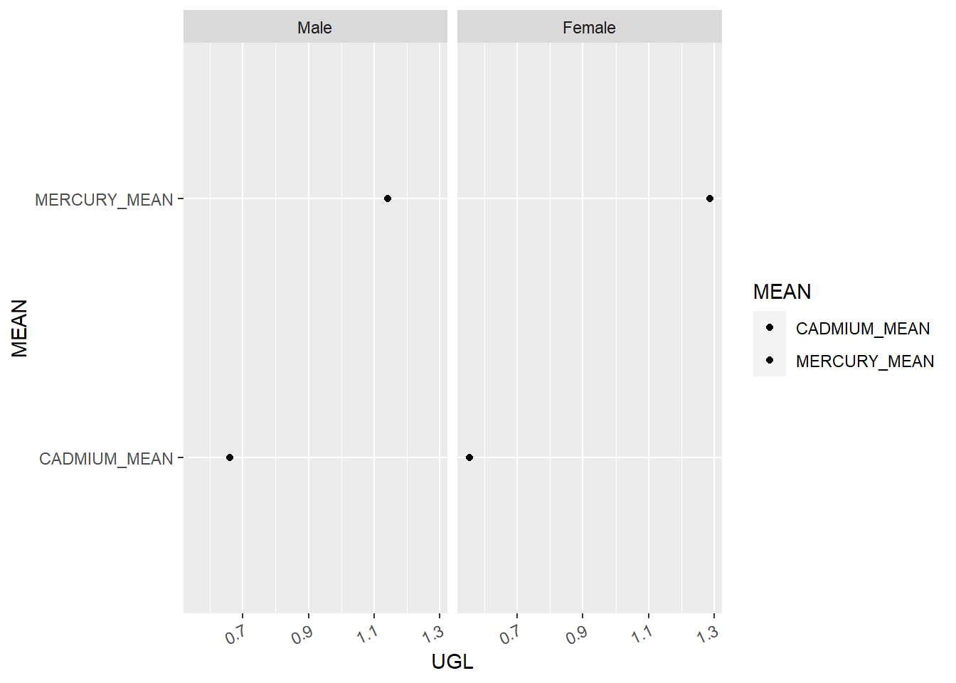
Heavy Metal Average: Between Male & Female
Code
#finding the average of heavy metals in males and females avg_metal <- final_select%>% dplyr::select(GENDER, DEPRESSED, CADMIUM_UGL, MERCURY_UGL)%>%group_by(GENDER)%>%filter(DEPRESSED ==1)%>%summarise(CADMIUM_MEAN =mean(CADMIUM_UGL, na.rm =TRUE),MERCURY_MEAN =mean(MERCURY_UGL, na.rm =TRUE))avg_metal
# A tibble: 2 × 3
  GENDER CADMIUM_MEAN MERCURY_MEAN
  <fct>         <dbl>        <dbl>
1 Male          0.661         1.14
2 Female        0.555         1.29
   SEQN AGE GENDER DEPRESSED CADMIUM_UGL MERCURY_UGL
1 39533  65 Female         0        0.63        0.48
2 41434  36 Female         0        0.20        1.03
3 37256  53   Male         1        0.28        0.39
4 40773  72   Male         0        0.23        2.75
5 40718  82   Male         0        0.54        0.78
6 31709  39   Male         0        0.56        1.51
Training Data
We decided to impute the missing values with median as the MAX data points were far from the majority of data points based on the quantiles.
Code
#decide to use Median over mean, as the 'Max.' are very far from spreadsummary(train)
      SEQN            AGE           GENDER     DEPRESSED  CADMIUM_UGL
 Min.   :31131   Min.   :18.00   Male  :1870   0:3031    Min.   : 0.1400
 1st Qu.:33800   1st Qu.:27.00   Female:1995   1: 834    1st Qu.: 0.2000
 Median :36309   Median :43.00                           Median : 0.3200
 Mean   :36328   Mean   :45.08                           Mean   : 0.5078
 3rd Qu.:38893   3rd Qu.:61.00                           3rd Qu.: 0.5800
 Max.   :41473   Max.   :85.00                           Max.   :10.8000
                                                         NA's   :154
  MERCURY_UGL
 Min.   : 0.140
 1st Qu.: 0.470
 Median : 0.880
 Mean   : 1.437
 3rd Qu.: 1.650
 Max.   :33.200
 NA's   :154
Code
train<-train %>% tidyr::replace_na(list(CADMIUM_UGL =median(train$CADMIUM_UGL,na.rm=TRUE),MERCURY_UGL =median(train$MERCURY_UGL,na.rm=TRUE)))#validation that NA are replaced by median sum(is.na(train))
[1] 0
Evaluation Metric
F1 score is a commonly used and effective evaluation metric for classification problems, especially when the dataset is imbalanced.
Our dataset presented an imbalance between the depressed and non-depressed individuals.
KNN
We tested for different values of k in k-nearest neighbors (KNN) models; k = 1 - 10.
k = 1 gave the best F1 score of 0.9904793
Code
train<-train%>%relocate(GENDER,DEPRESSED,.before=SEQN)set.seed(2)ctrl <-trainControl(method ="cv", number =5)#scale the datax <- train%>% dplyr::select( AGE:MERCURY_UGL)y<-train%>% dplyr::select(GENDER, DEPRESSED)x_scaled<-scale(x, center =TRUE, scale =TRUE)x_scaled<-cbind(y,x_scaled)k_list <-data.frame(matrix(ncol =2, nrow =10))colnames(k_list) <-c('K','F1')for (i in1:10) {KNN1 <-train(DEPRESSED~., data = x_scaled, tuneGrid=data.frame(k=i),method ="knn", trControl=ctrl, tuneLength =0)KNN1.pred<-predict(KNN1,x_scaled)cm_KNN1<-confusionMatrix(KNN1.pred,x_scaled$DEPRESSED,mode="prec_recall")f1 <- cm_KNN1$byClass["F1"]k_list[i, 1] <- ik_list[i, 2] <- f1}k_list
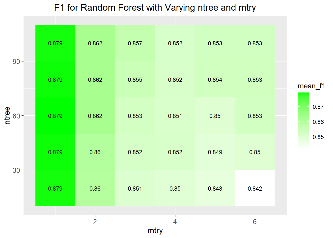
20 to 100 trees with an increment of 20 in our random forest model
6 different hyper-parameter control values 1 -6
Regardless of the number of trees, the best F1 score was obtained through the hyper-parameter value of 1.
Code
# set the seed for reproducibilityset.seed(2)# define the number of folds for cross-validationnum_folds <-5# define hyperparameters to optimizentree_values <-seq(20, 100, by =20)mtry_values <-c(1, 2, 3, 4, 5, 6)# initialize variables for storing performanceresults <-data.frame(ntree =numeric(),mtry =numeric(),mean_f1 =numeric(),SD_f1 =numeric() )# loop over hyperparameters to find the best combination and store performancefor (ntree in ntree_values) {for (mtry in mtry_values) {# initialize variable for storing performance across folds f1 <-numeric(num_folds)# loop over folds for cross-validationfor (fold in1:num_folds) {# create training and validation sets for current fold validIndex <- ((fold -1) * (nrow(train) / num_folds) +1):(fold * (nrow(train) / num_folds)) valid <- train[validIndex, ] train_rf <- train[-validIndex, ]# fit the random forest model with the current hyperparameters on the training set model <-randomForest(DEPRESSED ~ GENDER + AGE + CADMIUM_UGL + MERCURY_UGL,data = train_rf, ntree = ntree, mtry = mtry)# Make predictions on test data predictions <-predict(model, newdata = valid)# Create a confusion matrix confusion_matrix <-confusionMatrix(predictions, reference = valid$DEPRESSED)# Extract the confusion matrix metrics precision <- confusion_matrix$byClass["Pos Pred Value"] recall <- confusion_matrix$byClass["Sensitivity"] f1[fold] <-2* (precision * recall) / (precision + recall) }# calculate mean and standard deviation of RMSLE across folds mean_f1 <-mean(f1) SD_f1<-sd(f1)# store the performance of the current combination of hyperparameters results <-rbind(results, data.frame(ntree = ntree, mtry = mtry, mean_f1 = mean_f1, SD_f1 = SD_f1))print(paste('Completed mtry = ', mtry, 'and ntree = ', ntree))print(Sys.time()) }}
# print the optimal values of hyperparametersbest <- results[which.min(results$mean_f1), ]cat("Optimal ntree value:", best$ntree, "\n")
Optimal ntree value: 20
Code
cat("Optimal mtry value:", best$mtry, "\n")
Optimal mtry value: 6
Code
cat("Mean f1:", best$mean_f1, "\n")
Mean f1: 0.8415664
Code
ggplot(results, aes(x = mtry, y = ntree, fill = mean_f1)) +geom_tile() +scale_fill_gradient(low ="white", high ="green") +geom_text(aes(label =round(mean_f1, 3)), size =3, colour ="black") +ggtitle("F1 for Random Forest with Varying ntree and mtry") +xlab("mtry") +ylab("ntree") +theme(plot.title =element_text(size =14, hjust =0.5),axis.title =element_text(size =12),axis.text =element_text(size =10))
Support Vector Machine svmRadial
We observed a sequence of values from 0.1 to 1 with an increment of 0.1 for the width of the RBF kernel. Additionally, we observed a sequence of values from 1 to 10 with an increment of 1 for the regularization parameter in our SVM.
Best Parameters: sigma = 0.8, C = 1
F1 Score: 0.881435029896456
Code
set.seed(2)# Define the parameter gridparameter_grid <-expand.grid(sigma =seq(0.1, 1, by =0.1),C =seq(1, 10, by =1))# Train the SVM model with different parameter combinationssvm_model <-train(DEPRESSED ~ GENDER + AGE + CADMIUM_UGL + MERCURY_UGL, data = train, method ="svmRadial",trControl = ctrl, preProcess =c("center", "scale"),tuneGrid = parameter_grid, metric ="F1", maximize =TRUE)# Make predictions on the test datapredictions <-predict(svm_model, newdata = train)# Create a confusion matrixconfusion_matrix <-confusionMatrix(predictions, reference = train$DEPRESSED)# Extract the F1 scoref1_score <- confusion_matrix$byClass["F1"]# Print the best parameter combination and the corresponding F1 scoreprint(paste("Best Parameters: sigma =", svm_model$bestTune$sigma, "C =", svm_model$bestTune$C))
[1] "Best Parameters: sigma = 0.8 C = 1"
Code
print(paste("F1 Score:", f1_score))
[1] "F1 Score: 0.881435029896456"
Support Vector Machine svmLinear
We observed a sequence of values from 1 to 10 with an increment of 1 for the regularization parameter in our SVM.
Best Parameter: C = 1
F1 Score: 0.879060324825986
Code
set.seed(2)# Define the parameter gridparameter_grid <-expand.grid(C =seq(1, 10, by =1))# Train the SVM model with different parameter combinationssvm_model <-train(DEPRESSED ~ GENDER + AGE + CADMIUM_UGL + MERCURY_UGL, data = train, method ="svmLinear",trControl = ctrl, preProcess =c("center", "scale"),tuneGrid = parameter_grid, metric ="F1", maximize =TRUE)# Make predictions on the test datapredictions <-predict(svm_model, newdata = train)# Create a confusion matrixconfusion_matrix <-confusionMatrix(predictions, reference = train$DEPRESSED)# Extract the F1 scoref1_score <- confusion_matrix$byClass["F1"]# Print the best parameter combination and the corresponding F1 scoreprint(paste("Best Parameter: C =", svm_model$bestTune$C))
[1] "Best Parameter: C = 1"
Code
print(paste("F1 Score:", f1_score))
[1] "F1 Score: 0.879060324825986"
KNN for all Training Data
Code
set.seed(2)#scale the datax <- train%>% dplyr::select( AGE:MERCURY_UGL)y<-train%>% dplyr::select(GENDER, DEPRESSED)x_scaled<-scale(x, center =TRUE, scale =TRUE)x_scaled<-cbind(y,x_scaled)KNN_fin <-train(DEPRESSED~., data = x_scaled, tuneGrid=data.frame(k=1),method ="knn")KNN_fin.pred<-predict(KNN_fin,x_scaled)cm_KNN_fin<-confusionMatrix(KNN_fin.pred,x_scaled$DEPRESSED,mode="prec_recall")f1 <- cm_KNN_fin$byClass["F1"]f1
       F1
0.9911417
Test Data
We decided to impute the missing values with median as the max data points were far from the majority of data points based on the quantiles.
Code
set.seed(2)test<-test%>%relocate(GENDER,DEPRESSED,.before=SEQN)#decide to use Median over mean, as the MAX are vary far from spreadsummary(test)
    GENDER    DEPRESSED      SEQN            AGE         CADMIUM_UGL
 Male  :457   0:738     Min.   :31144   Min.   :18.00   Min.   :0.1400
 Female:509   1:228     1st Qu.:33854   1st Qu.:27.00   1st Qu.:0.2000
                        Median :36481   Median :43.00   Median :0.3300
                        Mean   :36413   Mean   :44.29   Mean   :0.5317
                        3rd Qu.:38998   3rd Qu.:60.00   3rd Qu.:0.5600
                        Max.   :41466   Max.   :85.00   Max.   :5.7100
                                                        NA's   :38
  MERCURY_UGL
 Min.   : 0.140
 1st Qu.: 0.470
 Median : 0.915
 Mean   : 1.436
 3rd Qu.: 1.730
 Max.   :20.900
 NA's   :38
Code
test<-test %>% tidyr::replace_na(list(CADMIUM_UGL =median(test$CADMIUM_UGL,na.rm=TRUE),MERCURY_UGL =median(test$MERCURY_UGL,na.rm=TRUE)))#validation that NA are replaced by median sum(is.na(test))
set.seed(2)knn_predictions <-predict(KNN_fin, newdata = test)# Create a confusion matrix for the test predictionsknn_confusion_matrix <-confusionMatrix(knn_predictions, reference = test$DEPRESSED)# Extract the F1 score from the test confusion matrixknn_f1_score <- knn_confusion_matrix$byClass["F1"]# Print the F1 score for the test setprint(paste("KNN F1 Score:", knn_f1_score))
[1] "KNN F1 Score: 0.846153846153846"
Code
set.seed(2)rf_fin <-randomForest(DEPRESSED ~ GENDER + AGE + CADMIUM_UGL + MERCURY_UGL,data = train_rf, ntree =20, mtry =1)rf_predictions <-predict(rf_fin, newdata = test)# Create a confusion matrix for the test predictionsrf_confusion_matrix <-confusionMatrix(rf_predictions, reference = test$DEPRESSED)# Extract the F1 score from the test confusion matrixrf_f1_score <- rf_confusion_matrix$byClass["F1"]# Print the F1 score for the test setprint(paste("Random Forest F1 Score:", rf_f1_score))
[1] "Random Forest F1 Score: 0.866197183098592"
Code
set.seed(2)svmrad_model <-train(DEPRESSED ~ GENDER + AGE + CADMIUM_UGL + MERCURY_UGL, data = train, method ="svmRadial",trControl = ctrl,preProcess =c("center", "scale"),tuneLength =1, # Set the number of hyperparameter combinations to 1tuneGrid =data.frame(sigma =0.8, C =1), # Set sigma and C valuesmetric ="F1",maximize =TRUE)# Make predictions on the test datasvmrad_predictions <-predict(svmrad_model, newdata = test)# Create a confusion matrix for the test predictionssvmrad_confusion_matrix <-confusionMatrix(svmrad_predictions, reference = test$DEPRESSED)# Extract the F1 score from the test confusion matrixsvmrad_f1_score <- svmrad_confusion_matrix$byClass["F1"]# Print the F1 score for the test setprint(paste("SVM Radial F1 Score:", svmrad_f1_score))
[1] "SVM Radial F1 Score: 0.864896755162242"
Code
set.seed(2)svmlin_model <-train(DEPRESSED ~ GENDER + AGE + CADMIUM_UGL + MERCURY_UGL, data = train, method ="svmLinear",trControl = ctrl,preProcess =c("center", "scale"),tuneLength =1, # Set the number of hyperparameter combinations to 1tuneGrid =data.frame(C =1), # Set the value for Cmetric ="F1",maximize =TRUE)# Make predictions on the test datasvmlin_predictions <-predict(svmlin_model, newdata = test)# Create a confusion matrix for the test predictionssvmlin_confusion_matrix <-confusionMatrix(svmlin_predictions, reference = test$DEPRESSED)# Extract the F1 score from the test confusion matrixsvmlin_f1_score <- svmlin_confusion_matrix$byClass["F1"]# Print the F1 score for the test setprint(paste("SVM Linear F1 Score:", svmlin_f1_score))
[1] "SVM Linear F1 Score: 0.866197183098592"
Comparing Models
KNN:
Overfitting and Underfitting:
KNN can suffer from overfitting when the value of k is too small, leading to excessive complexity and potentially memorizing the training data. On the other hand, with a large value of k, KNN may underfit and fail to capture the underlying patterns in the data.
Bias vs Variance Tradeoff:
KNN tends to have low bias but can have high variance, especially when k is small. As k increases, the model becomes more biased but also reduces its variance.
Flexibility vs Interpretability:
KNN is a flexible model that can capture complex relationships in the data. However, it is less interpretable compared to other models as it relies on the similarity of data points rather than explicit rules or coefficients.
In our project, k = 1 gave the best F1 score of 0.9904793. This suggests our model is overfitted and has low bias with high variance. As the value of our k value increases the F1 score decreases.
Random Forest:
Overfitting and Underfitting:
Random Forests are less prone to overfitting due to the ensemble nature of combining multiple decision trees. However, it can still overfit if the number of trees is very large or if individual trees are allowed to grow excessively deep.
Bias vs Variance Tradeoff:
Random Forests strike a balance between bias and variance by aggregating multiple decision trees. The individual trees in the ensemble tend to have high variance but when combined, the overall model has lower variance.
Flexibility vs Interpretability:
Random Forests offer a good balance between flexibility and interpretability. They can capture complex interactions in the data while also providing feature importances for interpretability.
In our project we observed 20 to 100 trees with an increment of 20 in our random forest model and 6 different hyper-parameter control values of 1 -6. Regardless of the number of trees, the best F1 score was obtained through the hyper-parameter value of 1. As the number of individual trees increase, we notice how our F1 scores decrease, which may suggest that the model does not suffer much overfitting.
However, we find it interesting that the F1 scores remain consistent when we increment our trees by 20 from 20 - 100. This observation can be further studied to better the random forest model.
SVM (Radial):
Overfitting and Underfitting:
SVM with a radial kernel can be prone to overfitting if the kernel parameters, such as sigma, are not properly tuned. If the kernel parameters are chosen poorly, the model may fail to generalize well to unseen data.
Bias vs Variance Tradeoff:
SVM with a radial kernel can have a high flexibility and may capture complex patterns in the data. However, if the model is excessively flexible due to incorrect parameter choices, it can have high variance.
Flexibility vs Interpretability:
SVM with a radial kernel is more flexible and can capture non-linear relationships in the data. However, the resulting model may be less interpretable compared to linear models.
In our project, we observed a sequence of values from 0.1 to 1 with an increment of 0.1 for the width of the RBF kernel. Additionally, we observed a sequence of values from 1 to 10 with an increment of 1 for the regularization parameter in our SVM.
SVM (Linear):
Overfitting and Underfitting:
SVM with a linear kernel is less prone to overfitting compared to models with more flexible kernels. However, it can still overfit if the regularization parameter (C) is set too small or if the data has a large number of features compared to the number of samples.
Bias vs Variance Tradeoff:
SVM with a linear kernel tends to have lower variance but can have a higher bias compared to more flexible models. It relies on finding the optimal hyperplane to separate the classes, which may not capture complex relationships.
Flexibility vs Interpretability:
SVM with a linear kernel strikes a balance between flexibility and interpretability. It can capture linear relationships in the data while providing interpretable coefficients for each feature.
We observed a sequence of values from 1 to 10 with an increment of 1 for the regularization parameter in our SVM. SVM with a radial kernel are more prone to overfitting when compared to SVM with a linear kernel. In general, SVM with a radial kernel is more flexible and can capture non-linear data more aptly. However, in our model we notice how the svmRadial and svmLinear approaches yield virtually the same F1 scores. This could suggest that the data contains linear relationships.
In summary, the Random Forest model generally performs well in terms of overfitting and bias-variance tradeoff due to its ensemble nature. SVM with a linear kernel and KNN also show similar performance in terms of overfitting and bias-variance tradeoff. However, Random Forest and SVM with a radial kernel offer more flexibility in capturing complex patterns, while SVM with a linear kernel provides better interpretability with its coefficients.
Ethical Consideration
HIPAA Violation:
With the understanding of heavy metals in urine and blood as a predictor of depression, a provider may have bias towards their patients. If a patient received labs for blood or urine analysis, the test may show the levels of heavy metals in their samples. A provider who observes the presence of the metals may form (un)conscious biases towards their patients. This could lead to potential HIPAA violations if a provider that is not in the scope of practice decided to investigate patients’ non-disclosed mental health status.
Hazard Transparency:
Heavy metals are commonly bio-accumulated through inhalation. Trace amounts of these metals can be IN THE AIR. Workers who are at higher risk of heavy metal inhalation due to their work environment should be properly informed of risk. If predictions between heavy metals and depression are known but obscured from employees, the workers may develop mental health concerns due to their work environment, but be unaware.
Concluding Remarks
We found that there is a statistically significant effect of Cadmium and Mercury between depressed and non-depressed groups. While running the models on the training set, KNN performed the best. However, when we compared the models using the test set, the difference in the F1 scores was minor, though the svmLinear performed slightly better.
Sources Referenced:
ChatGPT, personal communication, May 23, 2023
Oskar S, Stingone JA. Machine Learning Within Studies of Early-Life Environmental Exposures and Child Health: Review of the Current Literature and Discussion of Next Steps. Curr Environ Health Rep. 2020 Sep;7(3):170-184. doi: 10.1007/s40572-020-00282-5. PMID: 32578067; PMCID: PMC7483339.
Posit team (2023). RStudio: Integrated Development Environment for R. Posit Software, PBC, Boston, MA. URL http://www.posit.co/.
Xia F, Li Q, Luo X, Wu J. Machine learning model for depression based on heavy metals among aging people: A study with National Health and Nutrition Examination Survey 2017-2018. Front Public Health. 2022 Aug 4;10:939758. doi: 10.3389/fpubh.2022.939758. PMID: 35991018; PMCID: PMC9386350.
Xihang Fu, Huiru Li, Lingling Song, Manqiu Cen, Jing Wu, Association of urinary heavy metals co-exposure and adult depression: Modification of physical activity, NeuroToxicology, Volume 95,2023,Pages 117-12 ISSN 0161-813X,https://doi.org/10.1016/j.neuro.2023.01.008
Source Code
---title: "Mind your metals: Exploring the Impact of Heavy Metals on Depression with Machine Learning"editor: visualdate: "05/23/23"author: "Mekhala Kumar & Roy Yoon"format: html: toc: true code-fold: true code-copy: true code-tools: truetags: - NHANES - Depression - Heavy metal - Kumar - Yoon - AI---```{r setup}#| label: setup#| warning: false#| message: falselibrary(tidyverse)library(ggplot2)library(plotly)library(gapminder)library(readr)library(foreign)library(dplyr)library(reticulate)library(psych)library(caret)library(randomForest)library(MASS)library(e1071)library(yardstick)library(tidymodels)knitr::opts_chunk$set(echo =TRUE, warning=FALSE, message=FALSE)```# Mind Your Metals: Exploring the Impact of Heavy Metals on Depression with Machine Learning# National Health and Nutrition Examination Survey 2005-2006The *National Health and Nutrition Examination Survey* (NHANES) is a large and comprehensive dataset that includes information about the health and nutrition status of individuals in the United States. The 2005-2006 dataset (ICPSR 25504) is a nationally representative sample of individuals aged 6 months and older who participated in the survey between 2005 and 2006.The dataset includes a wide range of variables, including demographic information (age, sex, race/ethnicity, education level), health status (including chronic health conditions and health behaviors such as smoking and physical activity), and measures of nutrition and dietary intake (such as calorie and nutrient intake, dietary patterns, and food frequency). There are also physical measurements such as blood pressure, body mass index (BMI), and waist circumference.The dataset can be used to answer a wide range of research questions related to public health and nutrition. Some potential insights that can be gained from exploring the dataset include:- The prevalence of chronic health conditions such as hypertension, diabetes, and obesity in different demographic groups- The associations between health behaviors (such as smoking and physical activity) and health outcomes- The dietary patterns and nutrient intake of different demographic groups- The relationships between nutrition and health outcomes such as cardiovascular disease and diabetes- The associations between physical measurements such as BMI and waist circumference and health outcomesExploring these and other questions can provide valuable insights into the health status of different populations and can inform public health policies and interventions aimed at improving health outcomes.# Mind Your Metals: Exploring the Impact of Heavy Metals on Depression with Machine LearningThe association between heavy metals and depression has been a topic of interest in scientific research. Studies have investigated the potential relationship between exposure to heavy metals and the development or exacerbation of depressive symptoms. Here are some general observations from the existing literature:1. **Lead**: Exposure to lead has been associated with an increased risk of depressive symptoms. Lead is a neurotoxic metal that can affect the central nervous system and disrupt neurotransmitter function, potentially contributing to depressive symptoms.2. **Mercury**: Some studies suggest a possible link between mercury exposure and depression. Mercury is a toxic metal that can accumulate in the body, including the brain. It may have adverse effects on mood regulation and neurotransmitter function, potentially contributing to depressive symptoms.3. **Cadmium**: Cadmium exposure has been associated with an increased risk of depression in some studies. Cadmium is a toxic metal found in industrial pollutants and tobacco smoke. It may disrupt neuroendocrine function and contribute to the development of depressive symptoms.## Machine Learning within Studies of Early-life Environmental Exposures and Child Health: Review of the current literature and discussion of next-steps[Oskar and Stingone](https://www.ncbi.nlm.nih.gov/pmc/articles/PMC7483339/) emphasize that while ML methods have been widely used for prediction and classification in other fields, environmental health research has traditionally focused on causal or explanatory modeling. However, with the availability of complex environmental health data and the interest in holistic exposure paradigms such as the exposome, there is a need for analytic methods that can address the unique challenges posed by high-dimensional environmental health data.Their article explores how researchers have applied ML methods in studies of environmental exposures and childrens' health. It identifies common themes in these studies, including the analysis of environmental mixtures, exposure prediction and characterization, disease prediction and forecasting, analysis of other complex data, and improvements to causal inference. The review summarizes the strengths and limitations of implementing ML methods in these areas and identifies gaps in the literature.## Machine learning model for depression based on heavy metals among aging people: A study with National Health and Nutrition Examination Survey 2017--2018[Xia et al.](https://www.ncbi.nlm.nih.gov/pmc/articles/PMC9386350/) aimed to explore the association between depression and blood metal elements using a machine learning model. The study utilized data from the National Health and Nutrition Examination Survey (NHANES) conducted in 2017-2018. A total of 3,247 aging samples were included, and 10 different metals were analyzed, including lead (Pb), mercury (Hg), cadmium (Cd), manganese (Mn), selenium (Se), chromium (Cr), cobalt (Co), inorganic mercury (InHg), methylmercury (MeHg), and ethyl mercury (EtHg).The study compared eight machine learning algorithms for analyzing the association between metal elements and depression. Among the algorithms tested, XGBoost showed optimal effects and was used for further analysis. The study employed both Poisson regression and the XGBoost model to identify risk factors and predict depression.The results revealed that out of the 3,247 participants, 344 individuals were diagnosed with depression. In the Poisson regression model, the metals Cd (β = 0.22, P = 0.00000941), EtHg (β = 3.43, P = 0.003216), and Hg (β = -0.15, P = 0.001524) were found to be significantly related to depression. The XGBoost model demonstrated good performance for evaluating depression, with an accuracy of 0.89 (95%CI: 0.87, 0.92), a Kappa value of 0.006, and an area under the curve (AUC) of 0.88. An online XGBoost application for depression prediction was also developed.The study concluded that blood heavy metals, particularly Cd, EtHg, and Hg, were significantly associated with depression. The prediction of depression using machine learning models was deemed essential.## Association of urinary heavy metals co-exposure and adult depression: Modification of physical activity[Fu et al.](https://www.sciencedirect.com/science/article/abs/pii/S0161813X23000165) aimed to investigate the association between exposure to a mixture of urinary heavy metals and depression, as well as the potential moderating role of physical activity in this relationship. The study used data from the National Health and Nutrition Examination Survey (NHANES) conducted between 2011 and 2016. Depression was assessed using the Patient Health Questionnaire. Elastic net regression was used to select six heavy metals (cadmium, cobalt, tin, antimony, thallium, and mercury) for further analysis. Binomial logistic regression, generalized additive models, environment risk score (ERS), and weighted quantile sum (WQS) regression were employed to examine the effects of individual and cumulative exposure to these metals on depression risk. The study included 4,212 participants, and the prevalence of depression was 7.40%.The findings of the study indicated that urinary tin and antimony exposure were independently associated with an increased risk of depression. A linear dose-response relationship between tin exposure and depression risk was also observed. Moreover, cumulative exposure to multiple heavy metals was positively associated with depression risk, with tin, antimony, and cadmium identified as the metals contributing most to the overall mixture effect. Notably, the significant positive association between heavy metal mixture exposure and depression risk was observed primarily in individuals who were inactive in physical activity.In conclusion, this study demonstrated that combined exposure to urinary heavy metals was associated with an increased risk of depression. However, the detrimental effects of heavy metal exposure on depression risk appeared to be attenuated by engaging in physical activity. These findings have important implications for public health, highlighting the potential role of both heavy metal exposure and physical activity in the development and prevention of depression.# **Research Question:**- *Mind Your Metals* aims to predict how factors such as age, gender, and heavy metals(lead, cadmium, and mercury etc.) can have an affect on one's mental health, specifically depression. We will examine this topic as a classification problem.From the *National Health and Nutrition Examination Survey* we chose to examine:## [**Independent Variable(s):**]{.underline}- **DS1: Demographics** - Age - Gender- **DS102: Blood Lead and Blood Cadmium** - Lead - Cadmium- **DS130: Blood Total Mercury and Blood Total Inorganic Mercury** - Mercury - Inorganic Mercury## [**Dependent Variable**]{.underline}- **DS209: Depression Screener** - Feeling down, depressed, or hopeless# Exploratory Data Analysis## Tidying Data### **DS1: Demographics**```{r demographic}# demographic datademographic <-read.dta("sleep/DS0001/25504-0001-Data.dta")head(demographic)demographic_select <- demographic%>% dplyr::select(SEQN, RIAGENDR, RIDAGEYR)%>%rename(GENDER = RIAGENDR,AGE = RIDAGEYR)```### DS102: Blood Lead and Blood Cadmium```{r blood lead and cadmium}blood_PBCD <-read.dta("sleep/DS0102/25504-0102-Data.dta")head(blood_PBCD)blood_PBCD_select <- blood_PBCD%>% dplyr::select(SEQN, LBXBPB, LBXBCD)%>%rename(LEAD_UGDL = LBXBPB,CADMIUM_UGL = LBXBCD)```### DS130: Blood Total Mercury and Blood Inorganic Mercury```{r blood mercury and inorganic mercury}blood_HGIHG <-read.dta("sleep/DS0130/25504-0130-Data.dta")head(blood_HGIHG)blood_HGIHG_select <- blood_HGIHG%>% dplyr::select(SEQN, LBXTHG, LBXIHG)%>%rename(MERCURY_UGL = LBXTHG,INORG_MERCURY_UGL = LBXIHG)```### DS209: Depression Screener```{r depression}depression <-read.dta("sleep/DS0209/25504-0209-Data.dta")unwanted_categories <-c("Don't know", "Refused")depression_select <- depression%>% dplyr::select(SEQN, DPQ020)%>%rename(DEPRESSED = DPQ020)%>%filter(!(DEPRESSED %in% unwanted_categories))%>%filter(!is.na(DEPRESSED))depression_select$DEPRESSED<-droplevels(depression_select$DEPRESSED)depression_select <- depression_select%>%mutate(DEPRESSED =case_when( DEPRESSED =="Not at all"~0,TRUE~1 ))depression_select$DEPRESSED <-as.factor(depression_select$DEPRESSED)```## Join Data Frames```{r data frame select}head(demographic_select)head(blood_PBCD_select)head(blood_HGIHG_select)head(depression_select)``````{r join data}# merging demographic and blood lead and blood cadmiuma <- demographic_select %>%inner_join(blood_PBCD_select, by =join_by(SEQN))head(a)# merging demographic and blood lead and blood cadmium and blood total mercury and blood inorganic mercury b <- a %>%inner_join(blood_HGIHG_select, by =join_by(SEQN))head(b)# merging demographic and blood lead and blood cadmium and blood total mercury and blood inorganic mercury and depression screenerfinal_select <- b %>%inner_join(depression_select, by =join_by(SEQN))#LEAD_UGDL has a measurement tag of UGDL to correspond with the original NHANES data.head(final_select)```## Exploring Relationships## Summary Statistics```{r summary statistic}# 4831 rows and 8 columnsdim(final_select)print(summarytools::dfSummary(final_select,varnumbers =FALSE,plain.ascii =FALSE,style ="grid",graph.magnif =0.70,valid.col =FALSE),method ='render',table.classes ='table-condensed')```1. LEAD_UGDL: - Mean in group 0 (non-depressed): 1.816518 - Mean in group 1 (depressed): 1.811838 - The difference in means between the two groups is not statistically significant (p-value = 0.9397). The 95% confidence interval for the difference spans from -0.1166816 to 0.1260427.2. CADMIUM_UGL: - Mean in group 0 (non-depressed): 0.4885205 - Mean in group 1 (depressed): 0.5977713 - The difference in means between the two groups is statistically significant (p-value = 1.464e-06). The 95% confidence interval for the difference ranges from -0.15357010 to -0.06493149.3. MERCURY_UGL: - Mean in group 0 (non-depressed): 1.496233 - Mean in group 1 (depressed): 1.228055 - The difference in means between the two groups is statistically significant (p-value = 2.567e-06). The 95% confidence interval for the difference is between 0.1566488 and 0.3797086.4. INORG_MERCURY_UGL: - Mean in group 0 (non-depressed): 0.3450734 - Mean in group 1 (depressed): 0.3349219 - The difference in means between the two groups is not statistically significant (p-value = 0.2626). The 95% confidence interval for the difference spans from -0.007614401 to 0.027917506.These results suggest that there are statistically significant differences in the mean levels of CADMIUM_UGL and MERCURY_UGL between depressed and non-depressed groups. However, there are no significant differences in the mean levels of LEAD_UGDL and INORG_MERCURY_UGL between the two groups.```{r welch two sample t-test}t.test(LEAD_UGDL ~ DEPRESSED, data = final_select)t.test(CADMIUM_UGL ~ DEPRESSED, data = final_select)t.test(MERCURY_UGL ~ DEPRESSED, data = final_select)t.test(INORG_MERCURY_UGL ~ DEPRESSED, data = final_select)```## Heavy Metal Average: Between Male & Female```{r}#finding the average of heavy metals in males and females avg_metal <- final_select%>% dplyr::select(GENDER, DEPRESSED, CADMIUM_UGL, MERCURY_UGL)%>%group_by(GENDER)%>%filter(DEPRESSED ==1)%>%summarise(CADMIUM_MEAN =mean(CADMIUM_UGL, na.rm =TRUE),MERCURY_MEAN =mean(MERCURY_UGL, na.rm =TRUE))avg_metalavg_metal_pivot <-pivot_longer(avg_metal, CADMIUM_MEAN:MERCURY_MEAN, names_to ="MEAN", values_to ="UGL")avg_metal_pivotmf_avg_metal <-ggplot(data = avg_metal_pivot) +geom_point(mapping =aes(x =`MEAN`, y =`UGL`, fill =`MEAN`)) +theme(axis.text.x=element_text(angle=25,hjust=1)) +facet_wrap(~GENDER)+coord_flip()mf_avg_metal```# Data Split: Train(80%) and Test(20%)```{r split to train and test}final_select <- final_select%>% dplyr::select(SEQN, AGE, GENDER, DEPRESSED, CADMIUM_UGL, MERCURY_UGL)set.seed(2)train <- final_select %>%dplyr::sample_frac(0.8)test <- dplyr::anti_join(final_select, train, by ="SEQN")head(train)```# Training DataWe decided to impute the missing values with median as the MAX data points were far from the majority of data points based on the quantiles.```{r train}#decide to use Median over mean, as the 'Max.' are very far from spreadsummary(train)train<-train %>% tidyr::replace_na(list(CADMIUM_UGL =median(train$CADMIUM_UGL,na.rm=TRUE),MERCURY_UGL =median(train$MERCURY_UGL,na.rm=TRUE)))#validation that NA are replaced by median sum(is.na(train))```# Evaluation MetricF1 score is a commonly used and effective evaluation metric for classification problems, especially when the dataset is imbalanced.Our dataset presented an imbalance between the depressed and non-depressed individuals.## KNNWe tested for different values of k in k-nearest neighbors (KNN) models; k = 1 - 10.k = 1 gave the best F1 score of 0.9904793```{r KNN}train<-train%>%relocate(GENDER,DEPRESSED,.before=SEQN)set.seed(2)ctrl <-trainControl(method ="cv", number =5)#scale the datax <- train%>% dplyr::select( AGE:MERCURY_UGL)y<-train%>% dplyr::select(GENDER, DEPRESSED)x_scaled<-scale(x, center =TRUE, scale =TRUE)x_scaled<-cbind(y,x_scaled)k_list <-data.frame(matrix(ncol =2, nrow =10))colnames(k_list) <-c('K','F1')for (i in1:10) {KNN1 <-train(DEPRESSED~., data = x_scaled, tuneGrid=data.frame(k=i),method ="knn", trControl=ctrl, tuneLength =0)KNN1.pred<-predict(KNN1,x_scaled)cm_KNN1<-confusionMatrix(KNN1.pred,x_scaled$DEPRESSED,mode="prec_recall")f1 <- cm_KNN1$byClass["F1"]k_list[i, 1] <- ik_list[i, 2] <- f1}k_list```## Random ForestWe observed:1. 20 to 100 trees with an increment of 20 in our random forest model2. 6 different hyper-parameter control values 1 -6Regardless of the number of trees, the best F1 score was obtained through the hyper-parameter value of 1.```{r random forest}# set the seed for reproducibilityset.seed(2)# define the number of folds for cross-validationnum_folds <-5# define hyperparameters to optimizentree_values <-seq(20, 100, by =20)mtry_values <-c(1, 2, 3, 4, 5, 6)# initialize variables for storing performanceresults <-data.frame(ntree =numeric(),mtry =numeric(),mean_f1 =numeric(),SD_f1 =numeric() )# loop over hyperparameters to find the best combination and store performancefor (ntree in ntree_values) {for (mtry in mtry_values) {# initialize variable for storing performance across folds f1 <-numeric(num_folds)# loop over folds for cross-validationfor (fold in1:num_folds) {# create training and validation sets for current fold validIndex <- ((fold -1) * (nrow(train) / num_folds) +1):(fold * (nrow(train) / num_folds)) valid <- train[validIndex, ] train_rf <- train[-validIndex, ]# fit the random forest model with the current hyperparameters on the training set model <-randomForest(DEPRESSED ~ GENDER + AGE + CADMIUM_UGL + MERCURY_UGL,data = train_rf, ntree = ntree, mtry = mtry)# Make predictions on test data predictions <-predict(model, newdata = valid)# Create a confusion matrix confusion_matrix <-confusionMatrix(predictions, reference = valid$DEPRESSED)# Extract the confusion matrix metrics precision <- confusion_matrix$byClass["Pos Pred Value"] recall <- confusion_matrix$byClass["Sensitivity"] f1[fold] <-2* (precision * recall) / (precision + recall) }# calculate mean and standard deviation of RMSLE across folds mean_f1 <-mean(f1) SD_f1<-sd(f1)# store the performance of the current combination of hyperparameters results <-rbind(results, data.frame(ntree = ntree, mtry = mtry, mean_f1 = mean_f1, SD_f1 = SD_f1))print(paste('Completed mtry = ', mtry, 'and ntree = ', ntree))print(Sys.time()) }}# print the optimal values of hyperparametersbest <- results[which.min(results$mean_f1), ]cat("Optimal ntree value:", best$ntree, "\n")cat("Optimal mtry value:", best$mtry, "\n")cat("Mean f1:", best$mean_f1, "\n")ggplot(results, aes(x = mtry, y = ntree, fill = mean_f1)) +geom_tile() +scale_fill_gradient(low ="white", high ="green") +geom_text(aes(label =round(mean_f1, 3)), size =3, colour ="black") +ggtitle("F1 for Random Forest with Varying ntree and mtry") +xlab("mtry") +ylab("ntree") +theme(plot.title =element_text(size =14, hjust =0.5),axis.title =element_text(size =12),axis.text =element_text(size =10))```## Support Vector Machine svmRadialWe observed a sequence of values from 0.1 to 1 with an increment of 0.1 for the width of the RBF kernel. Additionally, we observed a sequence of values from 1 to 10 with an increment of 1 for the regularization parameter in our SVM.- Best Parameters: sigma = 0.8, C = 1- F1 Score: 0.881435029896456```{r svmRadial}set.seed(2)# Define the parameter gridparameter_grid <-expand.grid(sigma =seq(0.1, 1, by =0.1),C =seq(1, 10, by =1))# Train the SVM model with different parameter combinationssvm_model <-train(DEPRESSED ~ GENDER + AGE + CADMIUM_UGL + MERCURY_UGL, data = train, method ="svmRadial",trControl = ctrl, preProcess =c("center", "scale"),tuneGrid = parameter_grid, metric ="F1", maximize =TRUE)# Make predictions on the test datapredictions <-predict(svm_model, newdata = train)# Create a confusion matrixconfusion_matrix <-confusionMatrix(predictions, reference = train$DEPRESSED)# Extract the F1 scoref1_score <- confusion_matrix$byClass["F1"]# Print the best parameter combination and the corresponding F1 scoreprint(paste("Best Parameters: sigma =", svm_model$bestTune$sigma, "C =", svm_model$bestTune$C))print(paste("F1 Score:", f1_score))```## Support Vector Machine svmLinearWe observed a sequence of values from 1 to 10 with an increment of 1 for the regularization parameter in our SVM.- Best Parameter: C = 1- F1 Score: 0.879060324825986```{r svmLinear}set.seed(2)# Define the parameter gridparameter_grid <-expand.grid(C =seq(1, 10, by =1))# Train the SVM model with different parameter combinationssvm_model <-train(DEPRESSED ~ GENDER + AGE + CADMIUM_UGL + MERCURY_UGL, data = train, method ="svmLinear",trControl = ctrl, preProcess =c("center", "scale"),tuneGrid = parameter_grid, metric ="F1", maximize =TRUE)# Make predictions on the test datapredictions <-predict(svm_model, newdata = train)# Create a confusion matrixconfusion_matrix <-confusionMatrix(predictions, reference = train$DEPRESSED)# Extract the F1 scoref1_score <- confusion_matrix$byClass["F1"]# Print the best parameter combination and the corresponding F1 scoreprint(paste("Best Parameter: C =", svm_model$bestTune$C))print(paste("F1 Score:", f1_score))```## KNN for all Training Data```{r KNN for all of training data}set.seed(2)#scale the datax <- train%>% dplyr::select( AGE:MERCURY_UGL)y<-train%>% dplyr::select(GENDER, DEPRESSED)x_scaled<-scale(x, center =TRUE, scale =TRUE)x_scaled<-cbind(y,x_scaled)KNN_fin <-train(DEPRESSED~., data = x_scaled, tuneGrid=data.frame(k=1),method ="knn")KNN_fin.pred<-predict(KNN_fin,x_scaled)cm_KNN_fin<-confusionMatrix(KNN_fin.pred,x_scaled$DEPRESSED,mode="prec_recall")f1 <- cm_KNN_fin$byClass["F1"]f1```# Test DataWe decided to impute the missing values with median as the max data points were far from the majority of data points based on the quantiles.```{r test data clean}set.seed(2)test<-test%>%relocate(GENDER,DEPRESSED,.before=SEQN)#decide to use Median over mean, as the MAX are vary far from spreadsummary(test)test<-test %>% tidyr::replace_na(list(CADMIUM_UGL =median(test$CADMIUM_UGL,na.rm=TRUE),MERCURY_UGL =median(test$MERCURY_UGL,na.rm=TRUE)))#validation that NA are replaced by median sum(is.na(test))#scalex <- test%>% dplyr::select( AGE:MERCURY_UGL)y<-test%>% dplyr::select(GENDER, DEPRESSED)x_scaled<-scale(x, center =TRUE, scale =TRUE)x_scaled<-cbind(y,x_scaled)```## Prediction on Test Data- **KNN F1 Score**: 0.846153846153846- **Random Forest F1 Score**: 0.86454652532391- **SVM radial F1 Score**: 0.864896755162242- **SVM Linear F1 Score**: 0.866197183098592```{r Test Data Predictions1}set.seed(2)knn_predictions <-predict(KNN_fin, newdata = test)# Create a confusion matrix for the test predictionsknn_confusion_matrix <-confusionMatrix(knn_predictions, reference = test$DEPRESSED)# Extract the F1 score from the test confusion matrixknn_f1_score <- knn_confusion_matrix$byClass["F1"]# Print the F1 score for the test setprint(paste("KNN F1 Score:", knn_f1_score))``````{r Test Data Predictions2}set.seed(2)rf_fin <-randomForest(DEPRESSED ~ GENDER + AGE + CADMIUM_UGL + MERCURY_UGL,data = train_rf, ntree =20, mtry =1)rf_predictions <-predict(rf_fin, newdata = test)# Create a confusion matrix for the test predictionsrf_confusion_matrix <-confusionMatrix(rf_predictions, reference = test$DEPRESSED)# Extract the F1 score from the test confusion matrixrf_f1_score <- rf_confusion_matrix$byClass["F1"]# Print the F1 score for the test setprint(paste("Random Forest F1 Score:", rf_f1_score))``````{r Test Data Predictions3}set.seed(2)svmrad_model <-train(DEPRESSED ~ GENDER + AGE + CADMIUM_UGL + MERCURY_UGL, data = train, method ="svmRadial",trControl = ctrl,preProcess =c("center", "scale"),tuneLength =1, # Set the number of hyperparameter combinations to 1tuneGrid =data.frame(sigma =0.8, C =1), # Set sigma and C valuesmetric ="F1",maximize =TRUE)# Make predictions on the test datasvmrad_predictions <-predict(svmrad_model, newdata = test)# Create a confusion matrix for the test predictionssvmrad_confusion_matrix <-confusionMatrix(svmrad_predictions, reference = test$DEPRESSED)# Extract the F1 score from the test confusion matrixsvmrad_f1_score <- svmrad_confusion_matrix$byClass["F1"]# Print the F1 score for the test setprint(paste("SVM Radial F1 Score:", svmrad_f1_score))``````{r}set.seed(2)svmlin_model <-train(DEPRESSED ~ GENDER + AGE + CADMIUM_UGL + MERCURY_UGL, data = train, method ="svmLinear",trControl = ctrl,preProcess =c("center", "scale"),tuneLength =1, # Set the number of hyperparameter combinations to 1tuneGrid =data.frame(C =1), # Set the value for Cmetric ="F1",maximize =TRUE)# Make predictions on the test datasvmlin_predictions <-predict(svmlin_model, newdata = test)# Create a confusion matrix for the test predictionssvmlin_confusion_matrix <-confusionMatrix(svmlin_predictions, reference = test$DEPRESSED)# Extract the F1 score from the test confusion matrixsvmlin_f1_score <- svmlin_confusion_matrix$byClass["F1"]# Print the F1 score for the test setprint(paste("SVM Linear F1 Score:", svmlin_f1_score))```# **Comparing Models**1. KNN: - Overfitting and Underfitting: - KNN can suffer from overfitting when the value of k is too small, leading to excessive complexity and potentially memorizing the training data. On the other hand, with a large value of k, KNN may underfit and fail to capture the underlying patterns in the data. - Bias vs Variance Tradeoff: - KNN tends to have low bias but can have high variance, especially when k is small. As k increases, the model becomes more biased but also reduces its variance. - Flexibility vs Interpretability: - KNN is a flexible model that can capture complex relationships in the data. However, it is less interpretable compared to other models as it relies on the similarity of data points rather than explicit rules or coefficients. - In our project, k = 1 gave the best F1 score of 0.9904793. This suggests our model is overfitted and has low bias with high variance. As the value of our k value increases the F1 score decreases.2. Random Forest: - Overfitting and Underfitting: - Random Forests are less prone to overfitting due to the ensemble nature of combining multiple decision trees. However, it can still overfit if the number of trees is very large or if individual trees are allowed to grow excessively deep. - Bias vs Variance Tradeoff: - Random Forests strike a balance between bias and variance by aggregating multiple decision trees. The individual trees in the ensemble tend to have high variance but when combined, the overall model has lower variance. - Flexibility vs Interpretability: - Random Forests offer a good balance between flexibility and interpretability. They can capture complex interactions in the data while also providing feature importances for interpretability. - In our project we observed 20 to 100 trees with an increment of 20 in our random forest model and 6 different hyper-parameter control values of 1 -6. Regardless of the number of trees, the best F1 score was obtained through the hyper-parameter value of 1. As the number of individual trees increase, we notice how our F1 scores decrease, which may suggest that the model does not suffer much overfitting. - However, we find it interesting that the F1 scores remain consistent when we increment our trees by 20 from 20 - 100. This observation can be further studied to better the random forest model.3. SVM (Radial): - Overfitting and Underfitting: - SVM with a radial kernel can be prone to overfitting if the kernel parameters, such as sigma, are not properly tuned. If the kernel parameters are chosen poorly, the model may fail to generalize well to unseen data. - Bias vs Variance Tradeoff: - SVM with a radial kernel can have a high flexibility and may capture complex patterns in the data. However, if the model is excessively flexible due to incorrect parameter choices, it can have high variance. - Flexibility vs Interpretability: - SVM with a radial kernel is more flexible and can capture non-linear relationships in the data. However, the resulting model may be less interpretable compared to linear models. - In our project, we observed a sequence of values from 0.1 to 1 with an increment of 0.1 for the width of the RBF kernel. Additionally, we observed a sequence of values from 1 to 10 with an increment of 1 for the regularization parameter in our SVM.4. SVM (Linear): - Overfitting and Underfitting: - SVM with a linear kernel is less prone to overfitting compared to models with more flexible kernels. However, it can still overfit if the regularization parameter (C) is set too small or if the data has a large number of features compared to the number of samples. - Bias vs Variance Tradeoff: - SVM with a linear kernel tends to have lower variance but can have a higher bias compared to more flexible models. It relies on finding the optimal hyperplane to separate the classes, which may not capture complex relationships. - Flexibility vs Interpretability: - SVM with a linear kernel strikes a balance between flexibility and interpretability. It can capture linear relationships in the data while providing interpretable coefficients for each feature. - We observed a sequence of values from 1 to 10 with an increment of 1 for the regularization parameter in our SVM. SVM with a radial kernel are more prone to overfitting when compared to SVM with a linear kernel. In general, SVM with a radial kernel is more flexible and can capture non-linear data more aptly. However, in our model we notice how the svmRadial and svmLinear approaches yield virtually the same F1 scores. This could suggest that the data contains linear relationships.In summary, the Random Forest model generally performs well in terms of overfitting and bias-variance tradeoff due to its ensemble nature. SVM with a linear kernel and KNN also show similar performance in terms of overfitting and bias-variance tradeoff. However, Random Forest and SVM with a radial kernel offer more flexibility in capturing complex patterns, while SVM with a linear kernel provides better interpretability with its coefficients.# Ethical Consideration1. HIPAA Violation: 1. With the understanding of heavy metals in urine and blood as a predictor of depression, a provider may have bias towards their patients. If a patient received labs for blood or urine analysis, the test may show the levels of heavy metals in their samples. A provider who observes the presence of the metals may form (un)conscious biases towards their patients. This could lead to potential HIPAA violations if a provider that is not in the scope of practice decided to investigate patients' non-disclosed mental health status.2. Hazard Transparency: 1. Heavy metals are commonly bio-accumulated through inhalation. Trace amounts of these metals can be IN THE AIR. Workers who are at higher risk of heavy metal inhalation due to their work environment should be properly informed of risk. If predictions between heavy metals and depression are known but obscured from employees, the workers may develop mental health concerns due to their work environment, but be unaware.# Concluding RemarksWe found that there is a statistically significant effect of Cadmium and Mercury between depressed and non-depressed groups. While running the models on the training set, KNN performed the best. However, when we compared the models using the test set, the difference in the F1 scores was minor, though the svmLinear performed slightly better.# **Sources Referenced**:ChatGPT, personal communication, May 23, 2023Oskar S, Stingone JA. Machine Learning Within Studies of Early-Life Environmental Exposures and Child Health: Review of the Current Literature and Discussion of Next Steps. Curr Environ Health Rep. 2020 Sep;7(3):170-184. doi: 10.1007/s40572-020-00282-5. PMID: 32578067; PMCID: PMC7483339.Posit team (2023). RStudio: Integrated Development Environment for R. Posit Software, PBC, Boston, MA. URL http://www.posit.co/.Xia F, Li Q, Luo X, Wu J. Machine learning model for depression based on heavy metals among aging people: A study with National Health and Nutrition Examination Survey 2017-2018. Front Public Health. 2022 Aug 4;10:939758. doi: 10.3389/fpubh.2022.939758. PMID: 35991018; PMCID: PMC9386350.Xihang Fu, Huiru Li, Lingling Song, Manqiu Cen, Jing Wu, Association of urinary heavy metals co-exposure and adult depression: Modification of physical activity, NeuroToxicology, Volume 95,2023,Pages 117-12 ISSN 0161-813X,https://doi.org/10.1016/j.neuro.2023.01.008